Rules for selecting control valves

Nominal diameter

Control valves are never selected according to the diameter of the pipeline. However, the diameter of the pipeline before and after the valve must be calculated to select the piping of the control valves. Since the control valve is selected according to the Kvs value, often the nominal diameter of the valve is less than the nominal diameter of the pipeline on which it is installed, especially if there is a large difference across the valve. In this case, it is permissible to select a valve with a nominal diameter smaller than the nominal diameter of the pipeline by one or two stages. For larger differences, it is recommended to use valves with a reduced Kvs capacity. This solution allows us to reduce the cost of equipment, and with this selection, the equipment turns out to be more compact in size and weight.

w—recommended flow rate of the medium, m/s;
Q is the working volumetric flow rate of the medium m3/h;
d — pipeline diameter, m.

Control valve capacity kv/kvs

A control valve is a type of pipeline fitting most often used to regulate flow and pressure.
Correct selection of the control valve is a necessary condition for ensuring the normal operation of the piping system. Selection of a control valve comes down to determining its capacity at which a given excess pressure will be throttled at a given flow rate. The flow capacity of a control valve is characterized by the flow coefficient Kv. The Kv coefficient is equal to the flow rate of a working medium with a density of 1000 kg/m3 through the valve with a pressure drop across it of 0.1 MPa.

Formulas for determining the Kv coefficient differ for different types of media and pressure values; formulas for calculating Kv are presented in Table 1.

Table 1.

P1—pressure at the valve inlet, bar;
P2—pressure at the valve outlet, bar;
dP=P1 – P2 – pressure drop across the valve, bar;
t1—medium temperature at the inlet, 0C;
Q—liquid flow rate, m3/h;
Qn is the flow rate for gases at N.U., Nm3/h;
G—flow rate for water vapor, kg/h;
ρ - density kg/m3 (for gases, density at N.U. kg/nm3)

The Kv value is multiplied by the safety factor k1 (which is usually taken in the range of 1.2-1.3): Kvs=k1*Kv. And we get the value Kvs - the conditional capacity of the valve.

Based on the calculated Kvs value, according to the manufacturers' catalogs, a control valve with the closest possible Kvs value, taking into account the recommended diameter, is selected.

When selecting a control valve, it is also recommended to determine the nominal diameter of the valve and check for the occurrence of cavitation.

Nominal diameter of control valve

Control valves are never selected according to the diameter of the pipeline. However, the diameter must be determined to select the control valve trim. Since the control valve is selected according to the Kvs value, often the nominal diameter of the valve is less than the nominal diameter of the pipeline on which it is installed. In this case, it is permissible to select a valve with a nominal diameter smaller than the nominal diameter of the pipeline by one or two stages.

The calculated valve diameter is determined using the formula:

d—design valve diameter in, mm;
Q—medium consumption, m3/hour;
V – recommended flow speed m/s.

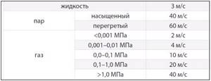
Recommended flow rate:

liquid – 3 m/s;
saturated steam – 40 m/s;
gas (at pressure <0.001 MPa) – 2 m/s;
gas (0.001 – 0.01 MPa) – 4 m/s;
gas (0.01 – 0.1 MPa) – 10 m/s;
gas (0.1 – 1.0 MPa) – 20 m/s;
gas (> 1.0 MPa) – 40 m/s;

Based on the calculated diameter value (d), the nearest larger nominal valve diameter DN is selected.

Checking the valve for cavitation

Cavitation is the process of formation and subsequent collapse of vacuum bubbles in a fluid flow, accompanied by noise and hydraulic shock, which in turn leads to premature wear of control valve elements.

To determine the possibility of cavitation occurring on the valve, the following condition is checked: dP ≤ 0.6P1.

Conditional pressure

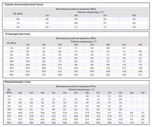
The nominal pressure Ru is the only parameter for manufactured fittings that guarantees its strength and takes into account both operating pressure and operating temperature. The conditional pressure corresponds to the permissible operating pressure for a given type of valve at normal temperature (20 °C). As the temperature rises, the mechanical properties of structural materials deteriorate, therefore, for valves with high operating temperatures, the permissible operating pressures are lower than the nominal ones. This reduction depends on the material of the reinforcement parts and the temperature dependence of the strength properties of this material. The higher the operating temperature, the lower the maximum operating pressure at the same nominal pressure value.

Below are tables of maximum operating pressure depending on temperature for various materials:

2.9. Calculation of control valves

Previous paragraph	Table of contents	Next paragraph
Return to literature selection

When calculating control valves, it is necessary to consider all the main characteristics and properties of the valve. This concerns the main issues of choosing the housing material, the stuffing box material, determining the nominal pressure and connecting dimensions. The selection process is the same as for conventional shut-off valves.

In addition, for control valves it is necessary to select an appropriate throttling system, taking into account the pressure drop and other conditions of medium flow through the valve (cavitation, evaporation of the medium, abrasive inclusions, flow of compressible fluids at a supercritical pressure drop, etc.), as well as a drive that to a certain extent affects the design of the valve (balanced, unbalanced, direct, reversible). The above is the main criterion for choosing a valve design.

Having made a choice, we can pay attention to calculating the regulating properties of the valve.

The main function of control valves is to regulate the flow or pressure loss in a piping system to a predetermined value by means of a variable flow coefficient. The control valves in an regulated system do not actually show the value of the flow coefficient Kvs for which it was designed, but the instantaneous value of the flow coefficient or losses that is set by the regulator after reaching the required regulated value. This means that at a particular moment the value of the flow coefficient is between zero (closed position) and a conditional value (fully open). The smoothness and fineness of regulation are set by the position of the operating point on the control characteristic of the controlled process, which means, as stated above, they largely depend on the instantaneous position of the operating point on the flow characteristic of the control valve and the entire system (significant influence of authority).

The operating curve of the consumer of the flowing medium, therefore, the dependence of the controlled variable on the flow rate of the medium through the consumer, determines the position of the operating point on the flow characteristic of the system. If there is no exact relationship, it is advisable to determine at least three main operating states at maximum, nominal and minimum fluid flow. The hydraulic pressure loss of the entire pipeline network, subtracted from the instantaneous available pressure difference at the source, determines, for a given selection, the available pressure at the control valve, which will be processed by this valve. It must be emphasized that the hydraulic loss of a pipeline system is not constant, but quadratically dependent on the flow rate of the medium through this system. It should be borne in mind that the source characteristic is also not constant, but, due to the internal resistance of the source, the available pressure drop across the source (pump head, etc.) drops. Based on the above, great care must be taken to determine the available pressure p at the control valve.

In each of the three states there will be a different pressure drop across the valve, so the Kv coefficient of the valve must be calculated separately for each of them. And only after discussing all the calculation results can we choose the Kvs coefficient of the valve. But first you need to answer the following questions:

— Is the calculated maximum flow through the valve really required?

— Is there a need to regulate this state further (increase the flow rate depending on other regulatory parameters)?

— What happens if the required flow rate is not achieved?

— Where is the operating point (stroke for the selected characteristic) of the valve when regulating the conditional flow?

— Where is the operating point of the valve when regulating the minimum quantity?

— Is it possible to regulate the maximum and minimum flow rates with one valve?

- What will happen if I am not able to regulate the minimum amount?

— What is better: not achieving the maximum or minimum expenses?

Although the previous questions may seem self-evident to experienced designers, they are useful to ask because they cover not only the calculation at conventional values, but also the actual operating condition at part load, which in practice creates quality problems regulation, especially in hot water installations.

And only now can we choose the Kvs value. If it is necessary to achieve maximum flow, we recommend increasing this value by 25 to 30%, which includes both a possible negative deviation of the maximum Kv value from Kvs (-10%) and deformation of the flow characteristic (hydraulic losses and source pressure drop, filter clogging , valve authority). Increasing the Kvs value is necessary in cases, especially in technological processes, when a certain ability to withstand overloads is required from the equipment.

In real practice in heating, on the contrary, it is more often recommended to choose the Kvs value that is the closest to the lowest, since often neither thermal nor hydraulic calculations are carried out, pressure and flow relationships, unfortunately, are guessed, and here the tendency to play it safe is manifested. If the first oversizing of the heating system begins when calculating heat losses, continues when choosing a heat-transfer surface, pipeline network, and ends with a heat source, then it is not surprising that the percentage overestimation of the heating system can be quite high. In addition, supply temperature or temperature gradient has a greater influence on power changes than flow. Therefore, the above-mentioned safety net turns out to be unnecessary. After selecting Kvs, it is advisable to check the control range of the valve. If the ratio Kvs/Kvs min

approaches or even exceeds the theoretical valve control ratio, you should consider how to avoid the minimum quantity control problem. First of all, it should be established whether there is a possibility of increasing the authority of the valve. There are two possibilities: increase the source pressure in the full power region or reduce hydraulic losses along the pipeline route. In the absence of such options, a higher quality valve with a higher control ratio (if available) should be used, or a minimum quantity control solution should be achieved using a smaller valve connected in parallel to the main valve (parallel valves).

The criteria for choosing a flow characteristic have already been mentioned earlier. First of all, care must be taken that the regulation works well and in its full range, that is, that the regulatory characteristic of the entire controlled process approaches an ideal linear relationship. If this is not possible, the priority operating state should be selected. The linear characteristic is more suitable for the area of higher relative flow rates and at high valve authority; on the contrary, it is advisable to use the equal percentage characteristic where good control sensitivity is required at low relative flow rates and at low valve authority. The parabolic relationship is a compromise between both of the above characteristics. The LDMspline characteristic is an optimized (the shape corresponds statistically most often to the characteristic of a water-water heat exchanger) version derived from the equal percentage characteristic, with the difference that it contains a deformation of the flow curve and, compared to the equal percentage characteristic, has higher sensitivity at the beginning and end of the stroke .

Previous paragraph	Table of contents	Next paragraph
Return to literature selection

Possibility of cavitation

One of the serious problems that arise when using shut-off and control valves is the occurrence of cavitation. This effect is especially pronounced when using regulators that reduce downstream pressure—reducing valves.

To check the possibility of cavitation occurring at large pressure drops across the valve, the following formula is used:

P1 – valve inlet pressure, bar;

∆P – pressure drop across the valve, bar.

Energy education

Selection of control valves

The principle of valve selection is common to all actuators of control devices (direct-acting temperature and pressure regulators, control valves with electric drives). It can also be used when selecting balancing, make-up (solenoid valves) and other pipeline fittings. The control valve must pass, in a cavitation-free and silent mode, the calculated amount of coolant through the heat-using system at the given coolant parameters, ensuring the required quality and accuracy of regulation (in conjunction with actuators and control devices).

Bandwidth

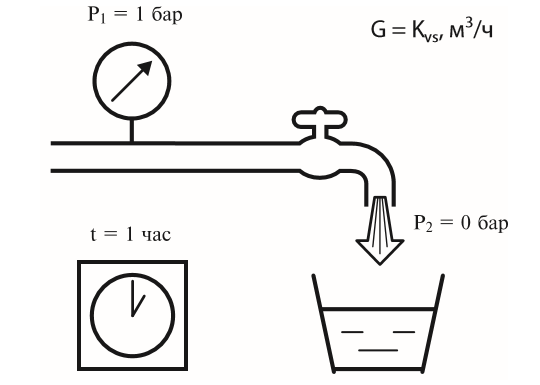
The selection of a control valve is based on its conditional capacity $K_{vs}$, which corresponds to the flow rate $G$ (m3/h) of cold water ($Т = 20$ °C) passing through a fully open valve with a pressure difference across it $ΔР_{cl.} = 1$ bar. $K_{vs}$ is a design characteristic of the valve. When selecting a valve, its $K_{vs}$ should be equal to or close to the required capacity value $K_v$ with the recommended margin:

$$K_{vs} ≥ K_v$$

Determination of the conditional capacity of the valve.

The required throughput is determined depending on the calculated coolant flow through the valve and the actual pressure drop across it according to the formula, m3/h:

$$K_v = \frac{1.2·G_p}{\sqrt{ΔР_{cl.}}}$$

where $G_р$ is the estimated coolant flow through the valve, m3/h; $ΔР_{cl.}$ — specified pressure drop across the valve, bar.

Estimated coolant flow

Heating and ventilation systems.

When determining the required capacity of a control valve for heating and ventilation systems, the calculated coolant flow rate $G_{рО(В)}$ is determined by their thermal load $Q_{О(В)}$ (kW) and temperature difference $ΔT = (Т_1 – T_2)$ in the circuit where the valve is installed, m3/h:
$$G_{pO(V)} = \frac{0.86·Q_{O(V)}}{T_1 – T_2}.$$
In this case, the temperature difference is taken according to the temperature chart at the calculated outside air temperature for heating design (for example, 150–70 °C).

DHW system.

The selection of control valves for DHW system heaters is carried out at the heating coolant flow rate, which is determined by the maximum hourly heat load on the DHW $Q_{DHW}$ (kW) and the temperature difference of the heating coolant at the break point of the temperature graph (for example, 70–40 ° C). The calculated coolant flow through the valve of the hot water system for direct water withdrawal from the heating network is taken in the amount of the maximum hourly flow of hot water for domestic and drinking needs or for the technological process.

The capacity of the valves of control devices that simultaneously serve the heating system and the domestic hot water system, for example, a pressure differential regulator common to these systems, is determined by:

for single-stage water heating for a hot water supply system - according to the sum of their estimated costs;
with a two-stage mixed water heating scheme (I stage of the water heater and the heating system are connected to the heating network in series, II stage - in parallel with the heating system) - based on the sum of the estimated costs for heating and hot water supply with a coefficient of 0.8.

Recharge system.

When choosing make-up devices, the calculated hourly flow rate is taken at 20% of the total volume of water in the heat consumption system, including the heater and expansion vessel. The volume of water in the heating system can be taken with sufficient accuracy at the rate of 15 liters for each kW of thermal power of the system.

Design pressure drop

Selecting the design pressure drop across control valves is the most difficult problem to solve. If the coolant flow through the valve is unambiguously specified, then the pressure drop across it can be varied. Not only the caliber of the valve, but also the performance and durability of the control device, the quietness of its operation, and the quality of regulation depend on the adopted pressure difference. The choice of pressure drop for all control valves of a heating point should be made comprehensively, in conjunction, taking into account specific conditions and the requirements given below. The initial value for selecting the pressure drop across the control valves of a heating point is the pressure difference in the pipelines of the heating network at the entrance to the building (at the input point of the heating point) $ΔР_с$. Typically, the pressure drop at the entrance to the building is taken according to the official data of the heat supply organization with a margin of 20% ($0.8·ΔР_с$). To ensure a high-quality regulation process and long-term operation of the control valve, the pressure drop across it must be greater than or equal to half the pressure drop in the regulated area:

$$ΔР^{open}_{cl} ≥ 0.5·ΔР_{р}$$

$$ΔР^{open}_{cl} ≥ Р{to}.$$

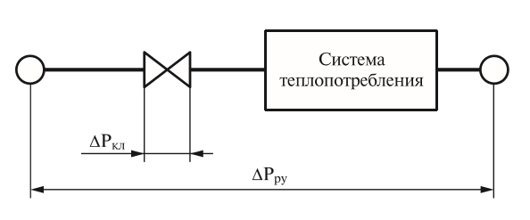
A regulated section is a part of a pipeline network with a heat-using installation where the valve is located, between points with a stabilized pressure difference or when it fluctuates within ±10%.

Selecting the differential pressure across the control valve.

The recommended absolute minimum pressure drop across the control valve is $ΔР^{min}_{cl} = 0.3$ bar. At the same time, the pressure drop across the valve should not exceed the maximum permissible value, which guarantees operation of the valve in cavitation-free mode. The valve should be checked for cavitation at the temperatures of the coolant passing through it. For this purpose, the maximum permissible pressure difference $ΔР^{prev}_{kl}$ is determined for the selected valve and compared with the accepted difference when calculating $K_v$. The maximum permissible pressure drop across the control valve is calculated using the formula, bar:

$$ΔР^{prev}_{cl} = Z·(P_1 – Р^{from b}_{sat.}),$$

where $Z$ is the cavitation onset coefficient. Accepted according to catalogs for control valves depending on their type and diameter; $P_1$ — coolant excess pressure in front of the control valve, bar; $P^{from b}_{sat.}$ is the excess pressure of saturated water vapor depending on its temperature $T_1$ in bar. If the calculated $ΔР^{prev}_{cl}$ turns out to be less than the previously accepted $ΔР_{cl}$, then it is necessary either to reduce the specified pressure drop across the valve by redistributing it between elements of the pipeline network, including through the additional installation of some either a throttling device (for example, a manual balancing valve) upstream of the valve, or move the valve to the return line where the coolant temperature is less than 100 °C. When using a non-pressure-balanced valve, the pressure drop across it must not exceed the limit value above which the valve will not close under the influence of an actuator with limited force. In all cases, in order to minimize noise generation, the pressure drop across the control valves is recommended to be no more than 2.5 bar.

Control valves in combination with electric drives have a relative control range of at least 1:30, i.e. the valve provides proportional control when the flow rate of the medium passing through it is reduced by 30 times compared to the $K_{vs}$ value. If you need to expand the control range, you can install two valves in parallel: one with a higher capacity, selected for the nominal flow rate of the coolant, and the second with a lower capacity, designed to pass 1/30 of the nominal flow. In this case, the electrical connections of the valves must be made in such a way that the “small” valve opens first, and only after it is fully opened, the “large” valve opens. To ensure this sequence of operation of the valves, their limit switches (built-in or additional) can be used. For a make-up system, the pressure drop across the solenoid valve is defined as the difference between the required static pressure in the heat consumption system when it is independently connected to the heating network and the pressure in front of the valve (in the return pipeline of the heating network or created by the make-up pump). The determination of design parameters and the sequence of selection of control valves are illustrated in the examples below.

Example 1

Select a control valve under the following conditions:

the valve is installed on the return pipeline after the heat-using installation;
coolant - water with a temperature in the return pipeline: $Т_2 = 70$ °C;
pressure loss in the heat-using installation (in the network): $ΔР_{to} = 1.5$ bar;
the available pressure in the regulated area is arbitrary (determined based on the results of valve selection);
calculated coolant flow: $G_р = 10$ m3/h.

Solution

1. Calculated pressure drop across the valve from the condition $ΔР_{кл} ≥ 0.5·ΔР_{ру}$, i.e.
$ΔР_{cl} ≥ ΔР_{to}$, is taken equal to $ΔР_у$, bar: $$ΔР_{cl} = ΔР_{to} = 1.5.$$
2. The required valve capacity is calculated using the formula, m3/h:

$$K_v = \frac{1.2·10}{\sqrt{1.5}} = 9.8.$$

3. A DN 25 valve with $K_{vs} = 10$ m3/h (the closest larger one to $K_v$) is selected from the technical catalogue.

Example 2

Select a control valve based on the following initial data:

coolant - water with temperature: $Т_1 = 150$ °C, and saturated vapor pressure: $Р_{us} = 3.85$ bar;
excess coolant pressure in front of the valve: $Р_1 = 7$ bar;
preset pressure drop across the control valve: $ΔР_{cl} = 2.5$ bar;
calculated coolant flow: $G_р = 40$ m3/h.

Solution

1. The required valve capacity is calculated using the formula, m3/h:
$$K_v = \frac{1.2·40}{\sqrt{2.5}} = 30.4.$$
2. From the catalog “Control valves with electric drives and hydraulic temperature controllers and pressure”, a valve DN 50 with $K_{vs} = 32$ m3/h and cavitation onset coefficient $Z = 0.5$ is preliminarily selected.

3. The maximum permissible pressure drop across the valve is calculated with a margin of 10%, bar:

$$ΔР^{prev}_{cl} = 0.5 · (7 – 3.85) · 0.9 = 1.4.$$

4. Since the initially accepted pressure drop across the valve turned out to be greater than the maximum permissible under cavitation conditions ($ΔР_{cl} = 2.5 > ΔР^{prev}_{cl} = 1.4$), $K^{tr}_{v} recalculated at $ΔР_{cl} = 1.4$ bar, m3/h:

$$K_v = \frac{1.2·40}{\sqrt{1.4}} = 40.6.$$

5. Based on the adjusted $K_v$ value, a DN 65 valve with $K_{vs} = 50$ m3/h and cavitation onset coefficient $Z = 0.5$ is selected.

Example 3

Select motor control valves and differential pressure regulator valves for the substation.

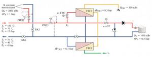
Heat point diagram.

Initial data:

The coolant is water supplied from a closed heating system according to a temperature schedule with a “summer” cutoff for hot water supply.
Estimated coolant temperature in the heating network: $Т_1 = 150$ °C and $Т_2 = 70$ °C. Temperature at the “break” point of the graph: $T'_1 = 70$ °C and $T'_2 = 40$ °C.
Excess pressure in the pipelines of the heating network: supply: $P_1 = 12$ bar, return: $P_2 = 4$ bar.
Estimated heat load: for heating: $Q_О = 1000$ kW, for ventilation: $Q_В = 2000$ kW, for DHW: $Q_{DHW} = 500$ kW.
Pressure loss: in the heating system: $∆Р_О = 0.5$ bar, in the ventilation system: $∆Р_В = 1$ bar, in the first stage of the DHW water heater (for heating water): $∆Р_{DHW1} = 0.3$ bar, in second stage of the DHW water heater (for heating water): $∆Р_{DHW2} = 0.2$ bar.

Solution

1. The estimated flow rate through the control valve in the coolant preparation unit for the heating system is calculated by the formula, m3/h:
$$G_{OT} = 0.86 · Q_O / (T_1–T_2) = 0.86 · 1000 / (150 – 70) = 10.75 .$$
2. Estimated flow rate through the differential pressure regulator valve for the ventilation system, m3/h:

$$G_B = 0.86 · Q_B / (T_1 – T_2) = 0.86 · 2000 / (150 – 70) = 21.5.$$

3. Estimated flow rate through the control valve of the DHW system, m3/h:

$$G_{DHW} = 0.86 · Q_{DHW} / (T'_1 – T'_2) = 0.86 · 500 / (70 – 40) = 14.33.$$

4. Estimated flow rate through the differential pressure regulator valve RPD1 for heating and hot water systems, m3/h:

$$G_{RPD1} = 0.8 · (G_O + G_{DHW}) = 0.8 · (10.75 + 14.33) = 20.06.$$

5. Maximum permissible pressure drop under the condition of non-cavitation operation on the valves of differential pressure regulators for heating systems with domestic hot water ($∆P^{max}_{RPD1}$) and ventilation systems ($∆P^{max}_{RPD2}$ ) at $Z = 0.5$ (recommended value for preliminary calculation) and $Р_{us} = 3.85$ bar, bar:

$$∆P^{max}_{RPD1} = ∆P^{max}_{RPD2} = Z · (Р_1 – Р_н) = 0.5 · (12 – 3.85) = 4.1.$$

6. We accept the pressure difference on the differential pressure regulators with a margin of 10%, bar:

$$∆Р_{RPD1} = ∆Р_{RPD2} = 0.9 · 4.1 = 3.7.$$

7. Pressure in the supply pipeline in front of the control valves of heating and hot water systems, bar:

$$Р_3 = Р_1 – ∆Р_{RPD1} = 12 – 3.7 = 8.3.$$

8. Maximum permissible pressure drop under the condition of non-cavitation operation on the control valves of the heating system ($∆Р_{klOT}$) and DHW ($∆Р_{klOT}$) with the previously accepted $Z = 0.5$ and $Р_{us} = $3.85 bar, bar:

$$∆Р^{max}_{clOT} = ∆Р^{max}_{clDHW} = Z · (Р_3 – Р_{sat}) = 0.5 · (8.3 – 3.85) = 2.2.$$

9. We accept the pressure drop on the valves of heating and hot water systems with a margin of 10%, bar:

∆Р_{cl.O} = ∆Р_{cl.DHW} = 0.9 2.2 = 2.

10. Excess pressure in the ring of heating and hot water systems is extinguished using the additional manual balancing valve BKI installed at the inlet, taking the available pressure at the inlet with a margin of 10%, bar:

$$∆Р_{БК1} = 0.9 · (Р_1 – Р_2) – ∆Р_{РПД1} – ∆Р_{cl.О} – ∆Р_{DHWI} = 0.9 · (12 – 4) – 3.7 – 2 – 0.3 = 1.2.$$

11. Excess pressure in the ventilation system ring is extinguished using an additionally installed manual balancing valve BK2, bar:

$$∆Р_{БК2} = 0.9 · (Р_1 – Р_2) – ∆Р_{БКI} – ∆Р_{РПД2} – ∆Р_В = 0.9 · (12 – 4) – 1.2 – 3.7 – 1 = 1.3.$$

12. Required capacity of control valves, m3/h:

for heating:

$$K_v = \frac{1.2·G_О}{\sqrt{∆Р_{cl.О}}} = \frac{1.2·10.75}{\sqrt{2}} = 9.14;$$

for DHW:

$$K_v = \frac{1.2·G_DHW}{\sqrt{∆Р_{DHW class}}} = \frac{1.2·14.33}{\sqrt{2}} = 12.2;$$

for RPD1:

$$K_v = \frac{1.2·G_RPD1}{\sqrt{∆Р_{RPD1}}} = \frac{1.2·20.06}{\sqrt{3.7}} = 12.54;$$

for RPD2:

$$K_v = \frac{1.2·G_В}{\sqrt{∆Р_{RPD2}}} = \frac{1.2·21.5}{\sqrt{3.7}} = 13.44.$$

13. Valves are selected from the catalog based on the required flow capacities: for heating: DN = 25 mm with $K_{vs} = 10$ m3/h and $Z = 0.5$; for DHW: DN = 32 mm with $K_{vs} = 16$ m3/h and $Z = 0.5$; for RPD1: DN = 32 mm with $K_{vs} = 16$ m3/h and $Z = 0.55$; for RPD2: DN = 32 mm with $K_{vs} = 16$ m3/h and $Z = 0.55$.

Noise level

When choosing a pressure regulator, it is necessary to take into account the phenomena associated with the noise of the operating regulator. The occurrence of noise is caused by gas-dynamic oscillatory processes near the regulators and the walls of the regulators. If the oscillation frequency coincides, the amplitude of the valve oscillations can increase sharply, which will lead to wear and destruction of the valve, as well as strong vibration of the regulator.

The main reason for the increased noise is the increased velocity of the medium in the selected pipeline relative to the recommended one. The actual speed of the medium can be calculated using the formula:

w – medium flow velocity, m/s;
Q – working volumetric flow rate of the medium m3/h;
d – pipeline diameter, m.

The following are recommended media speeds to reduce the risk of critical noise levels:

One of the ways to reduce the noise level in systems, in addition to the use of specially designed valves, is the use of flexible inserts (vibration compensators) in the areas before and after the valve.

How to select and apply three way valve

The three-way valve must be selected correctly for its capacity. It must also have the correct thread diameter (1/2 or 3/4 inch) and fit properly with the thermal head or servo.

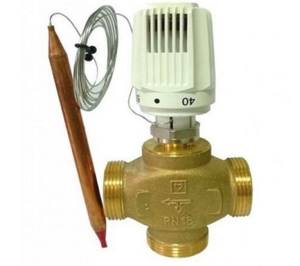
There are valve designs with a built-in temperature sensor, so it does not need a thermal head.

In the lists of companies’ equipment you can find a lot of devices of this type; from all this you have to choose what you need, which is not always easy. In many ways, knowledgeable specialists from a trading organization will help you make the right choice. But you should not rely only on their opinion; it is better to understand the issue yourself.

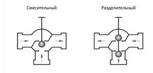
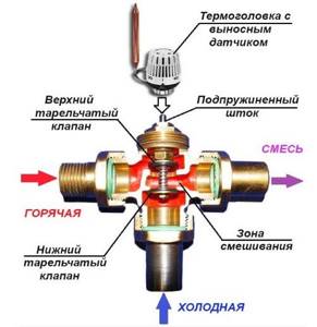
Mixing and separating three-way valves

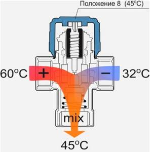
A three-way valve is a unit for mixing (separation) of liquid flows with three connections. Arrows on the valve body indicate the function it performs. For example, the device mixes 2 streams in different proportions depending on the position of the poppet valve.

In the first extreme position, only the first flow will reach the output, in the other extreme position, only the second flow, in the middle position, the flows will be mixed in equal proportions, for example.

If liquids with different temperatures are supplied, then using the valve it is possible to regulate the temperature of the liquid at the outlet, obtained as a result of mixing the two streams.

The separation valve will separate the flows into 2 directions, mixing coolant in one proportion or another into different branches. Its application is exactly the same as the mixing valve, only the installation along the branches is mirrored.

Based on both valves, it is possible to create temperature control units in heating networks. In this case, the outlet temperature can be adjusted by a built-in temperature sensor, or the valve can be controlled by a thermal head with an external temperature sensor.

Three-way valve designs

Seat valves are more commonly used, in which the seat moves on a spring-loaded stem and closes the inlet openings. This is a common design used with push-action thermal heads.

Another option is a rotary ball switch. Switching between flows occurs when the regulator is turned, which is usually done by a servo drive upon command from a temperature sensor. Such a system is more expensive and volatile.

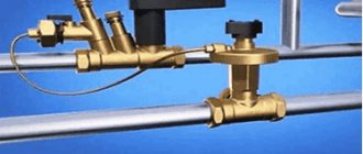
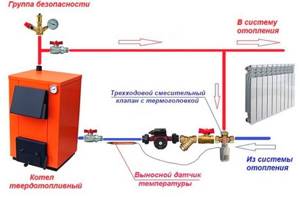
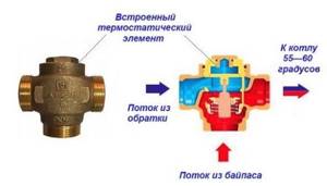
Application diagram of a three-way valve

A typical connection diagram for a three-way valve to protect the heat exchanger of a solid fuel boiler from cold return. The coolant is mixed from the supply to the return in a small circle. The goal is to always maintain a return temperature greater than 55 degrees, so that water vapor does not condense on the heat exchanger, and, accordingly, to avoid significant contamination and acid corrosion.

The bellows sensor of the thermal head is installed on the return line and gives a command to the thermal head about the degree of pressure on the rod of the seated three-way mixing valve. Pre-opening is adjusted by rotating the setting.

Where else are three-way valves used?

A typical application for adjusting the coolant temperature using three-way valves is as follows.

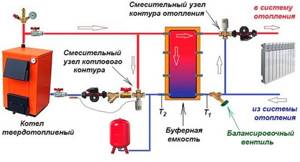
Adjusting the temperature of the coolant supplied from the buffer tank. A charged heat accumulator may contain too hot liquid that is not needed in the house. Therefore, the valve mixes cold return into the supply stream according to the owners’ settings.

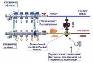
Maintaining coolant temperature in underfloor heating circuits. For normal operation of heated floors, the supply temperature should not exceed 55 degrees. Boilers for radiator networks usually produce more. In most underfloor heating schemes, pumping and mixing units are installed to maintain a stable temperature under pressure and coolant flow changes.

In complex heating circuits, where circuits with different temperature needs are connected after the pressure equalizer (buffer, water gun, ring). It is more reliable to perform the adjustment not by reducing the flow rate along the circuit, but by using a mixing unit based on a three-way valve.

Instead of a three-way valve, in many schemes a two-way valve can be used to regulate the amount of flow, which will then be mixed into the main stream at the tee. But these units require stable pressure, as well as special calculations, so a two-way valve can be found in factory pumping and mixing units.

Sometimes only a fixed outlet temperature is required. A valve with a thermostatic device is cheaper...

How to select a three-way valve based on capacity

The main characteristic of a three-way valve is its nominal flow capacity, designated as Kvs, m³/h. It is indicated subject to a pressure difference at the valve fittings of 1 bar.

For example, in the catalog (in the characteristics) you can find Kvs = 2.5 in m³/h, this means that at a pressure of 1 bar, 2.5 cubic meters of coolant will pass through a fully open valve in an hour. But how to use this figure in real conditions?

First, we need to find out how much liquid we need to pass through such a valve? Secondly, what will be the pressure drop across the valve in our circuit?

The required liquid flow rate Ktr, m3/hour through the valve for any circuit is not difficult to calculate using the formula:

Three-way valve calculation

Ktr = 0.86 Q/∆t, where Q is the power of the branch (heat load), for a boiler or heating circuit of the whole house is taken according to the heat generation power kW, ∆t is the difference in supply and return temperatures, usually 20 degrees, and for warm floor - 10 degrees.

Then, to piping a 20 kW boiler, liquids of at least Ktr = 0.86 20/20 = 0.86 m3/hour must pass through the valve, with a pressure drop of 1 bar.

But our pressure drop is much less - about 0.2 bar. At this pressure, the valve capacity should be significantly greater. Which exactly?

The pressure drop for any circuit between supply and return will not exceed 0.2 bar, typically in the range of 0.1 - 0.2 bar.

There is a certain empirical formula in this regard - the valve capacity in our circuit should be no less than

K= Ktr/√r, m cubic/hour, K= 0.86 / √0.2 = 1.9 m³/hour.

We select a valve with a higher characteristic: Kvs is greater than K, but not by much, so as not to overpay too much for the volume of the structure, Kvs = 2.5 m³/h is suitable.

We select a three-way mixing valve with this capacity from a well-known manufacturer and believe that it provides us with normal mixing in a circuit with a power of 20 kW.

In general, selecting thermal heads, their placement, and setting up work with the selected three-way or two-way valve is not such a simple task. For beginners, it is advisable to consult with at least an experienced seller with an installation demonstration and instructions for use, creating a mixing unit, and determining whether it is suitable for a specific scheme. Especially if you plan to use an electric drive. Or you can entrust this work to a specialist.

Ratio of inlet to outlet pressure or permissible pressure drop across the valve

Some pressure reducing valves have a limited inlet to outlet pressure ratio. The inlet pressure, acting on the plunger of the pressure reducing valve, tends to open it. The outlet pressure acts on the diaphragm (or other control element) of the valve, tending to close the valve. If the limit on the ratio of inlet to outlet pressure is exceeded, the valve will not be able to close - and the outlet pressure will be greater than the set pressure. Limitations on this parameter also eliminate cavitation in the control valve seat.

Following these instructions when selecting regulators will significantly improve the performance of technological processes and increase the service life of control valves. Examples of calculations are given in the article. For questions regarding the selection of equipment, please contact the engineers of the control valves department of ADL.

Valve adjustment range

Performing its function of controlling the flow of matter or energy, the control valve must ensure a change in flow rate within a given range. Let us determine the parameter of the flow characteristic, called the control range . This parameter is determined by the ratio of the maximum flow through the control valve to the minimum adjustable flow and is designated by the symbol εр (epsilon-er). The concept of “ minimum adjustable flow ” is not theoretically defined, but in practice it is generally accepted that the minimum adjustable flow is the flow rate at a valve valve stroke equal to 5% of the maximum (conditional) stroke. In accordance with this definition, for a linear flow characteristic the control range is 20.

However, in practice, the flow characteristic is not linear. Its shape is determined by two factors:

- the form of the throughput characteristic - the dependence of the throughput characteristic Kvy on the position (stroke) of the gate;

- a parameter of the pipeline system, determined by the ratio of the pressure drop in the line and across the control body when the valve is fully open (we denote this parameter by the symbol n ).

The parameter n is a characteristic of the pipeline system: how many hydraulic resistances it includes (technological devices, straight sections of pipelines, local resistances, shut-off valves), except for the control valve. If n = 0, then this means that the only resistance in the piping system is the control valve (a situation that is quite rare, but possible). Generally accepted practice dictates that the pressure drop across the control valve when it is fully open should not be less than 10% of the total pressure drop in the system (this is the limit!). This limit corresponds to n = 9.

When we talk about the shape of the throughput characteristic, we mean its parameter called the minimum throughput. We are talking about the throughput from which the regulatory process begins. And here we again use the “5% rule”: the minimum throughput is the throughput at a move equal to 5% of the maximum (conditional) move. The ratio of the conditional throughput Kvy to the minimum throughput is called the range of change in throughput; Let's denote this parameter by the symbol ε (epsilon). Thus, the range of change in throughput depends on the shape of the throughput characteristic. For linear throughput characteristic ε =20; for an equal percentage throughput characteristic it is customary to assume ε =50. You can use a special throttle pair with a higher throughput range. How much the value of this parameter can be increased depends on many factors (seat diameter, nominal stroke), but in the general case it seems possible to obtain the value ε = 100.

For a specific pipeline system, the control range εр depends on the range of change in throughput ε and on the ratio of drops n :

εр = f(ε,n)

For a liquid, for example, this relationship has the form:

From this rather simple relationship, important conclusions can be drawn:

— The control range εр is always less than the range of change in capacity ε .

— The control range εр for a valve with an equal percentage flow characteristic is approximately 2.5 times greater than for a valve with a linear characteristic.

— It seems possible to at least double the control range (compared to the equal percentage characteristic) by using a control valve with a special flow characteristic.

And finally, about the use of a double-seat valve in a situation where a high value of the control range is required. Due to the design features, the range of change in capacity for a double-seat valve does not exceed 25, regardless of the shape of the flow characteristic. Therefore, a high control range cannot be achieved with a double-seat control valve.